Tracking of color edges and blobs is key to the low computational load of our vision system. The idea is to utilize the fact that the world changes slowly, as compared to the frame rate. This makes it possible to predict the location where certain features will appear in the next frame. If most of these features are found close to their predicted positions, only small parts of the image need to be touched. The differences between the measured locations and the predictions can be used to update estimates of the parameters of a world model.
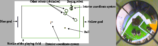
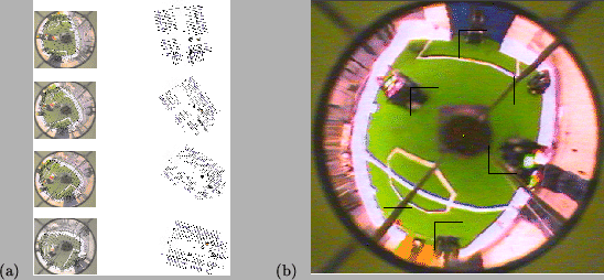
We use a 2D-model of the field, with the robots and the ball on it, as shown in Fig. 4. The model is matched sequentially to the video frames. For each model line, short orthogonal equidistant tracking lines form a tracking grid (Fig.5(a)).
 |
The ends of each tracking line specify two color classes, according to the expected colors at both sides of the line. Each tracking line is mapped into the image, using the inverse camera function. This is done by mapping the endpoints of each transition line into the image and then reconnecting them with a line. Next, the pixels along the projection line are searched for the appropriate color transition. In Figure 5(b) detected transitions are marked with a black dot. It can be seen that the model does not fit precisely to the playing field in the image, due to a rotation of the robot. Sometimes false transitions may be found, e.g. at field lines. They need to be detected as outliers that must be ignored.
The next step is to calculate a 2-D rigid body transformation that brings the model in correspondence with the found transitions. In the case here, the model should be rotated slightly to the left. To determine the model's transformation, first a rotation and translation is calculated for each track grid independently. Then the results are combined to obtain a transformation for the whole model.
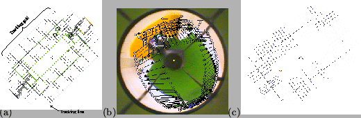
Repeating the above steps while perceiving a sequence of images yields the desired result: the pose of the field seen from the robots point of view is tracked and so the position and orientation of the robot is known by a simple coordinate transformation. Figure 6(a) shows the tracking while the robot rotates.
During initial search candidate positions are evaluated using the tracking mechanism. Given a position of the robot and the angle of a goal, the robot's orientation is calculated. The field can now be projected into the image and the ratio of found transitions can be used as quality measure for model fit. This ratio is also used during tracking to detect situations when the tracking fails and the initial search is needed to localize the robot again.
The system does not only track color edges, but also color blobs, such as the ball or obstacles. The blobs are only searched for in small square windows around their predicted positions, as shown in Fig. 6. If an object cannot be found within its rectangle, initial search is started to localize it again.